December 15, 2010

••• documentation


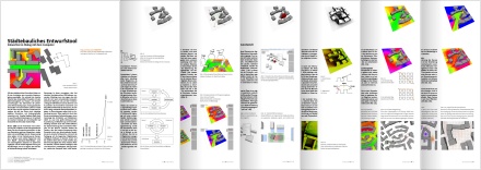
This is a little documentation of our spatial analyses tool for urban design (german)

With this project, we won the 1st price at the competition aufITgebaut 2011


you can download the file here (pdf, 1.3mb)
Labels: ,

November 7, 2010

••• spatial analyses for urban environments


A little demo video of the so far implemented features.

Labels: ,

November 1, 2010

••• swarm simulation


Here are a few more flocking experiments, exploring the performance and structure of a swarm with elements of different size and behaviour. There are four setups shown in the video:
  • All boids are of equal size and move with the same speed
  • The boids have different sizes, but move with the same speed
  • The boids have different sizes and act by different behaviours. Small boids are fast and agile, big boids are slow and lazy.
  • Generally all boids are equal. If they get compressed by many neighbors, they get bigger and faster. When the danger is over, they get normal again.

Labels: , ,

October 20, 2010

••• spatial analyses for urban environments


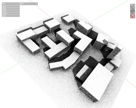
The aim of the project is to question the role of computer-aided design methods in urban development, to ask in which parts of the design process the use of the computer can be appropriate. While commonly the focus of most computer aided design sotware is on drawing layouts, that are defined by various analog methods, it does not give the designer any information about the quality of the design itself.

The developed tool assists the designer in an early step of the design process, where basic principles of the layout are defined. While the conditions of the design regarding light, spatial, geometrical and urbanistic context are displayed, it can be addapted in real-time.

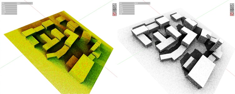
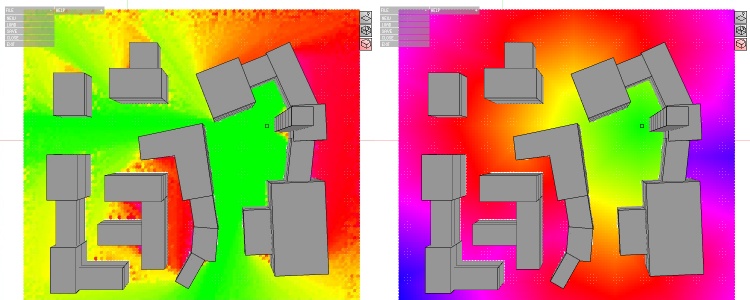
Therefore three kinds of analysis methods are implemented in the tool so far:


Illumination solver (left: Sun gradient - green=morning, red=evening, right: Static sun)


Accessibility solver (left: by angle, right: by distance)


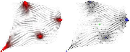
Spatial analysis solver

references/links:
Aedas, space syntax, kaisersrot

Labels: ,

October 18, 2010

••• depth of field


Depth of field blur effect in Processing with OpenGL.

There are two different types of materials: spriteMaterial for sprites, such as points, labels, ... and lineMaterial. You define these materials in void setup() (in this case 11 different types of points and one line type). You can actually convert any texture (image + alpha map) into a sprite material, in this example, there is only points and text.


you can download the source code here

Labels: ,

October 8, 2010

••• swarm simulation


Nature provides a various number of systems, that seem to be of immense complexicity and to act completely unpredictable. On the same time, these systems consist of elements, that follow comprehensible rules regarding to each other and to their environment.

The simulation of those system enables to explore their behaviour and potential regarding self organization and self optimization in design and architecture.

The boids (class boid - black points) move by these five rules:
  • do not get to close to any of your neighbors
  • try to swim in the same direction as the neighbors
  • don't leave the sphere
  • if you get lost: try to catch up with someone, who's around
  • run away from the shark

The sharks (class shark - red points) move by two rules:
  • swim in the direction, where the most boids are
  • don't leave the sphere

Labels: , ,

July 15, 2010

••• relaxation form finding 2


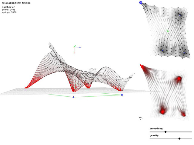
Second version of the form finding tool in processing. There are a few improvements to version one of the sketch:
  • triangulated point grid for more stability
  • points can move in x and z-direction now (only as long, as the structure is still buildable)
  • a better exporter, to wind up the bended girders. The sketch saves a pdf file for prototyping eg. on cnc laser cutting machines
Like in the first version of the sketch, the girder depth is calculated by the stress values of each point in the grid. While designing the form with the tool, you can see these values displayed in the stress map (take a look at the video above for a little demonstration).

height map (right), stress map (left)
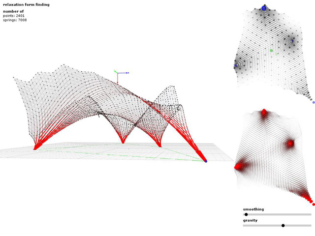
Screenshots

click for larger images

Labels: , ,